TimeSeries
TimeSeries objects are the focal point of the ursa library, contining much of the functionality required for performing fast and convenient timseries operations, creating new timeseries as a function of other timeseries, caching live timeseries data, upsampling, downsampling, and more.
Interfaces
Interfaces contain code for populating TimeSeries objects with data from a variety of marketplaces. Every interface objects contains both
A historical data interface, for retrieving historical data for the TimeSeries associated with that interface’s source,
And a live interface for harvesting live market data.
Historical data interfaces usually involve querying some REST endpoint of a market data provider.
Live data interfaces are sometimes also implemented to poll a REST webservice, however are usually more efficiently implemented as websocket streams (where avaialble / possible).
TimeSeries data is stored in two places:
A redis cache or redis cluster corresponding with your ursa instance
A timeseries database used to securely store the underlying timeseries data long-term.
Interfaces are still under development
We aim to soon build customizable interfaces, for the purpose of allowing users of ursa to develop custom base-level timeseries, however for now, if you’d like to implement a custom interface, you should code it up directly in the ursa library and submit a pull request on our github!
Live
Live interfaces are responsible for:
Reading in data from a webservice / websocket
Computing the correct timestamp bin where the newest data belongs
Updating the redis timeseries entry for the correct timestamp bin with the newest value which has been observed in the market
Updating the corresponding timestamp bin in any DataTable object which contains the relevant TimeSeries, or any children of that TimeSeries.
Historical
Historical interfaces are responsible for:
Querying a (usually REST) webservice endpoint from some market data provider
Computing the corresponding timestamp bins for the incomming historical data
Updating the database with historical data for the corresponding timeseries
TimeSeries.dataset()
TimeSeries.dataset() is where the data lives!
It’s nice to be able to create many TimeSeries objects, however the real power of ursa is in the immediate ability to track live datasets of your newly defined TimeSeries objects without any additional effort.
TimeSeries.dataset() is how you get your TimeSeries dataset as a Series object from either Pandas or Polars. It can be invoked like this:
Pandas
# Import required objects
from ursa_sync.backend import TimeSeries
from ursa_sync import session

# Open a session with the database
db = session()

# Load a TimeSeries object
TS = TimeSeries.load(4321, db)

# Access the TimeSeries data:
series = TS.dataset(format='pandas')
Polars
# Import required objects
from ursa_sync.backend import TimeSeries
from ursa_sync import session

# Open a session with the database
db = session()

# Load a TimeSeries object
TS = TimeSeries.load(1234, db)

# Access the TimeSeries data:
series = TS.dataset(format='polars')
Computed Features & Parent Child Hierarchy
TimeSeries objects are built with a parent / child hierarchy. This allows you to quickly build new timeseries as a function of other timeseries. There are two main types of TimeSeries objects:
Non Computed TimeSeries:
Non-Computed TimeSeries objects are defined such that:
TS.computed = False
By definition, a non-computed TimeSeries object may not have parents, as it is dirived from raw, unfiltered, uncomputed and unaltered market data.
Non-Computed TimeSeries have interfaces (as described above) for retrieving live and historical data.
Data corresponding with Non-Computed TimeSeries objects is stored in the database, and when active, the cache.
Computed TimeSeries:
Computed TimeSeries objects are defined as TimeSeries objects such that:
TS.computed = False
Computed TimeSeries do not have interfaces for collecting live nor historical data. Instead, they are computed from other TimeSeries (their “parents”).
Data Corresponding with Computed TimeSeries objects is NOT stored in the database, nor in the cache. Data instead is computed on-demand, when requested.
When dataset() is called on a computed TimeSeries, dataset() is called on all that TimeSeries’ parents, and grandparents, recursively until we can directly compute the dataset of TimeSeries.
The number of parents a Computed TimeSeries has is determined by the Compute Type of the TimeSeries (see below). In principle, there is neither a limit to the number of parents a TimeSeries can have, nor a limit to the generation depth that a grand-grand…parent/…/parent/child relationship can go. There are of course practical limits depending on your use case.
In the case that many large computations are necessary to compute a computed TimeSeries object’s data, it may take too long to actually compute to be considered useful for your use case.
In this case, you can pre-compute the computed TimeSeries by assigning it to an active DataTable, a table such that
DT.active == True
In this case, it will be computed upon data arriving for its parents, and cached directly in the DataTable’s cache dataset.
Compute Types
There are a variety of compute-types, which define the function which is used to compute the computed TimeSeries object’s data. A comprehensive list and corresponding descriptions of the various compute types can be found below:
Automatically-Created Compute Types
Below, are the compute-types which permit automatic creation of new TimeSeries objects via standard arithmetic operations.
These operations create a new object by simply performing simple arithmetic on TimeSeries objects. However, these operations do not store the resulting objects in the database / backend.
If you want to persist these objects in your instance beyond the working session, it is necessary to call TimeSeries.save() after constructing it.
Difference
A TimeSeries object can be created by subtracting one TimeSeries from another:
# Import required objects
from ursa_sync.backend import TimeSeries
from ursa_sync import session

# Open a session with the database
db = session()

TS1 = TimeSeries.load(1, db)
TS2 = TimeSeries.load(2, db)

# TS3 is now a TimeSeries object which will be automatically
# computed from TS1 and TS2's data.
TS3 = TS1 - TS2

# The call to TS3.save() will store the object in the database,
# so that it can persist beyond your current session.
# Upon calling TS3.save(), TS3 is assigned an id value.
TS3.save()
Similarly, you can create a new TimeSeries object as the difference between a TimeSeries object and any numeric value.
# TS4 is now also a new TimeSeries object.
TS4 = TS3 - 100

# Perhaps more usefully, we can attempt to create a stationary # TimeSeries by subtracting the mean from all values:
TS5 = TS3 - TS3.dataset().mean()

TS4.save()
TS5.save()

db.close()
Sum
Sum works in an identical fashion to difference.
TS3: ursa.backend.TimeSeries = TS1 + TS2
TS4: ursa.backend.TimeSeries = TS1 + 5
Product
So does Product. For exact details, see the section on “Difference”
TS3: ursa.backend.TimeSeries = TS1 * TS2
TS4: ursa.backend.TimeSeries = TS1 * 5
Division
Division works the same as above. For exact details, see the section on “Difference”
TS3: ursa.backend.TimeSeries = TS1 / TS2
TS4: ursa.backend.TimeSeries = TS1 / 5
Similarly, integer division is also compatible with TimeSeries objects (as with Difference):
TS3: ursa.backend.TimeSeries = TS1 // TS2
TS4: ursa.backend.TimeSeries = TS1 // 5
Greater Than or Equal
By using the python operation greater than or equal to, between two TimeSeries objects, or between a TimeSeries object and a numeric value, we construct a binary TimeSeries which takes on the value 1, when the inequality is satisfied, and a 0 when not.
For instance:
# This constructs a binary timeseries which is 1 whenever
# The dataset value of TS is greater than or equal to 0, and
# 0 in all other case.
TS3: ursa.backend.TimeSeries = TS >= 0

# Similaraly, you can create a binary TimeSeries indicating
# when one TimeSeries is greater than another:
TS3: ursa.backend.TimeSeries = TS >= TS2
Less Than or Equal
The same is true about the “less than or equal to” operator:
# This constructs a binary timeseries which is 1 whenever
# The dataset value of TS is less than or equal to 0, and
# 0 in all other case.
TS3: ursa.backend.TimeSeries = TS <= 0

# Similaraly, you can create a binary TimeSeries indicating
# when one TimeSeries is less than another:
TS3: ursa.backend.TimeSeries = TS <= TS2
Equal
A similar principal applies to the equality operator (see greater than or equal to for exact details):
TS3: ursa.backend.TimeSeries = TS == 0
TS3: ursa.backend.TimeSeries = TS == TS2
Not Equal
TS3: ursa.backend.TimeSeries = TS != 0
TS3: ursa.backend.TimeSeries = TS != TS2
Less Than
TS3: ursa.backend.TimeSeries = TS < 0
TS3: ursa.backend.TimeSeries = TS < TS2
Greater Than
TS3: ursa.backend.TimeSeries = TS > 0
TS3: ursa.backend.TimeSeries = TS > TS2
Manually-Created Compute Types
The creation of other computed TimeSeries requires some more careful specifications than simple arithmetic operations.
In this case, we provide a set of manually-specified compute types for building TimeSeries objects manually.
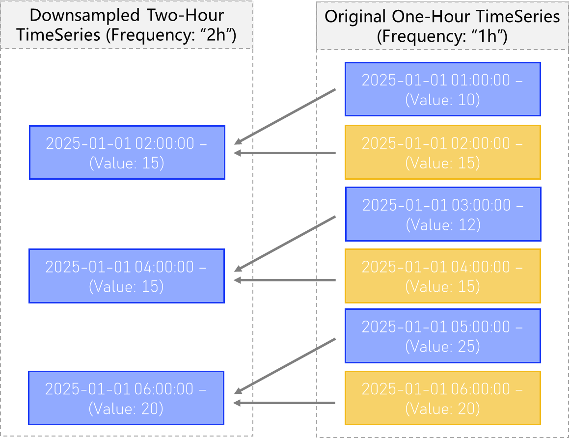
Downsample
Downsampling is a common operation related to TimeSeries management and construction.
Downsampling is the primary means by which we can change the “frequency” attribute of a TimeSeries object.
In general, child TimeSeries have the same value of TS.frequency as their parents, with the exception of upsampling and downsampling operations.
Downsample Types
There are a few different ways to define a downsampled timeseries. Valid downsample types can be found in the Enum class DownsampleTypes:
# Import the enum class to see valid DownsampleTypes
from ursa_sync.backend.cases.DownsampleTypes import DownsampleTypes

DownsampleTypes().types
Out:
['mean', 'expmean', 'sum', 'max', 'min', 'first', 'last', 'median']
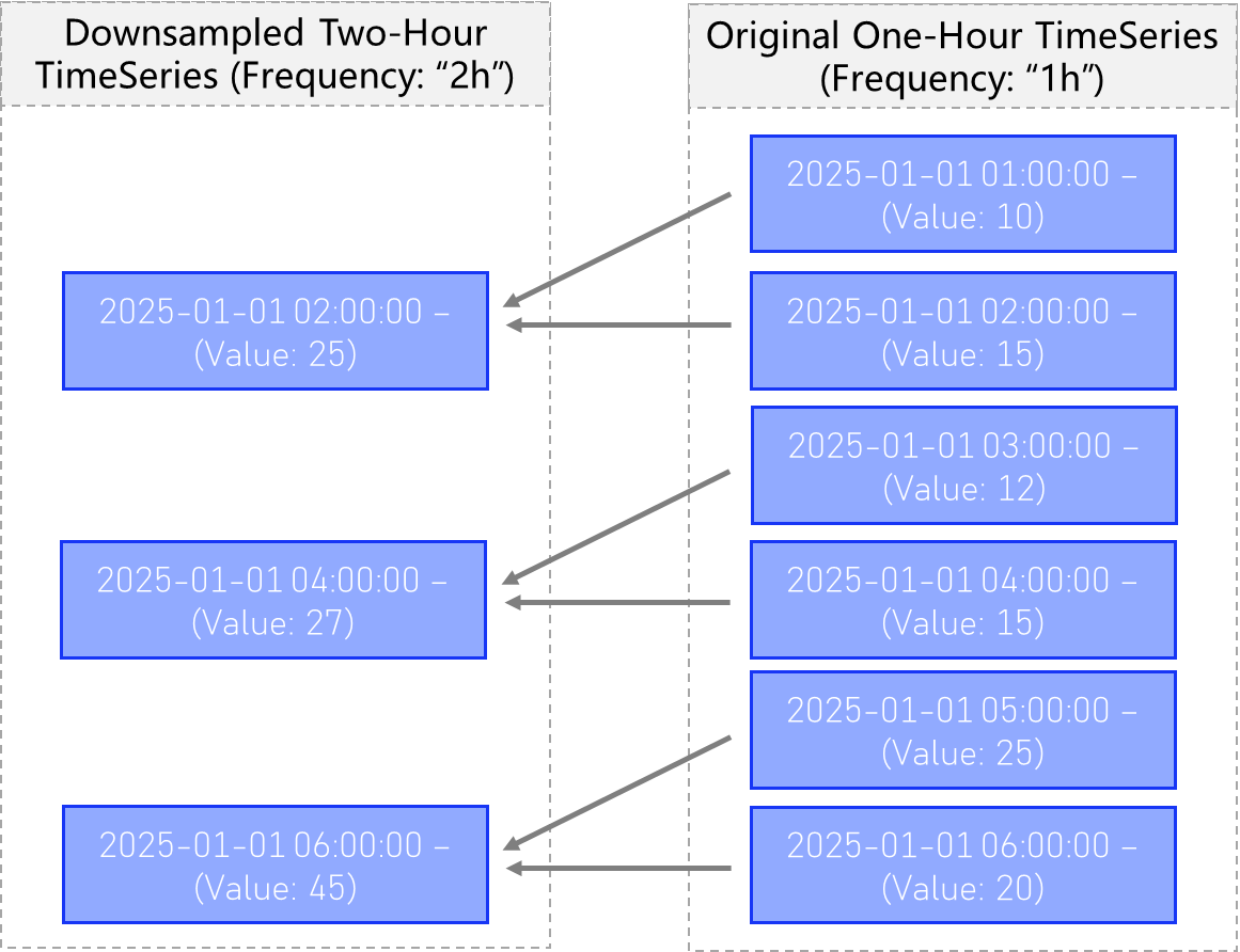
Sum
A Computed TimeSeries with downsample type “Sum”, will compute the sum of all values within each bin for the new frequency, and assign it to the new larger bin (see below).
Mean
A computed TimeSeries with downsample type “Mean”, will compute the mean of all values within each bin for the new frequency, and assign it to the new larger bin.
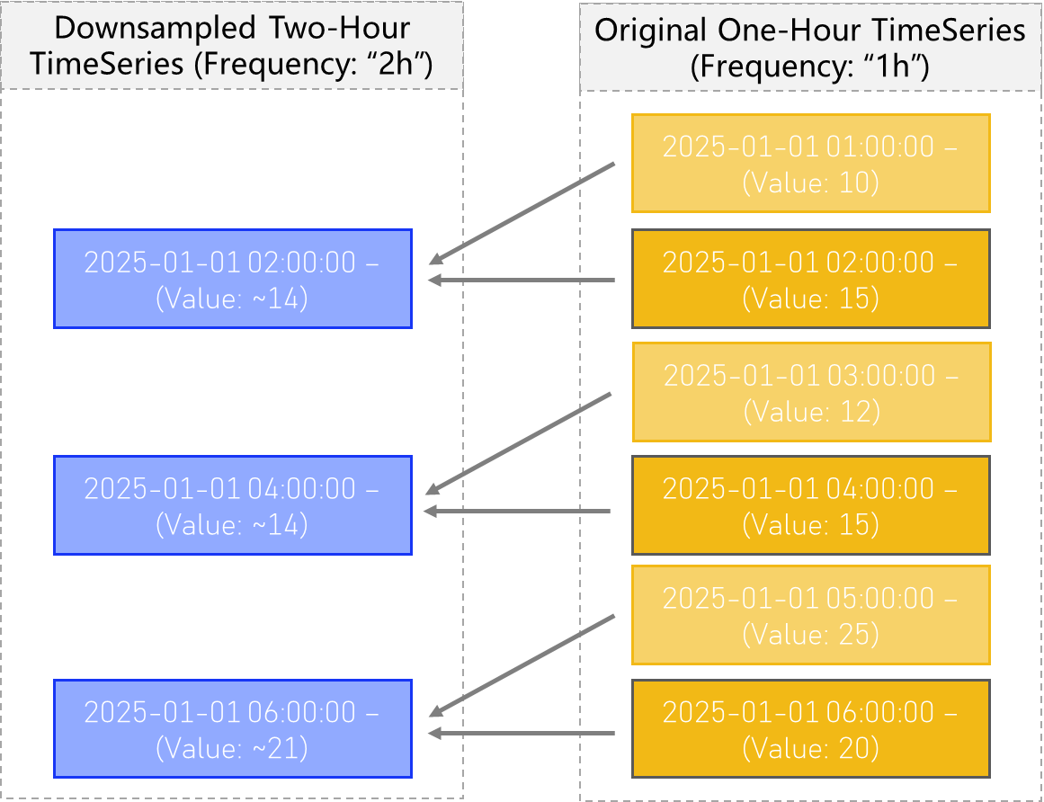
Exp Mean
A computed TimeSeries with downsample type Exp Mean (the exponentially-weighted mean) produces a downsampled TimeSeries which is similar to that of type Mean, except that observations closer to the end of the new time bins, contribute more to the overall average.
In this case, all observations are averaged together, but with weights corresponding to how recent, or close the observation is to the end of the new timestamp bins.
See the figure below for a visual explanation:
Median
The two-sample Median is the same as the Mean setting. However more generally, if the Median downsample type is specified, the new bins will be computed as the median value of all the old timestamp values falling within each respective bin.
Min
The downsample type of type “min” will take the minimum value observed in all the values associated with timestamps within the new TimeSeries’ time bins, and assign it that minimum value.
See below:
Max
Max functions exactly how you would expect, functioning the same as the min setting, but by using the maximum observed value instead of the minimum.
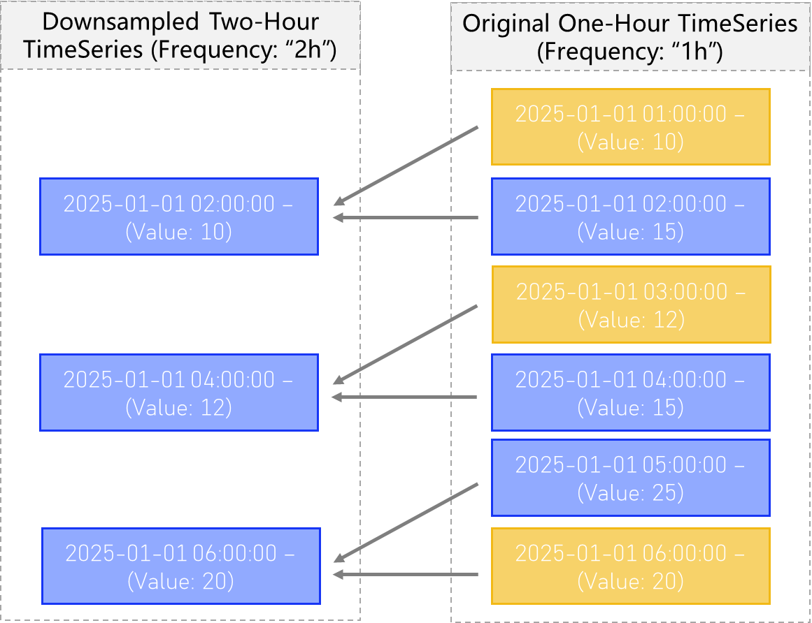
First
The “First” downsample setting will tell the downsampler to only use the first observed value, of all the timestamp values observed in the old time bins, and assign that value to the new bin without considering any following values.
This process can be visualized below:
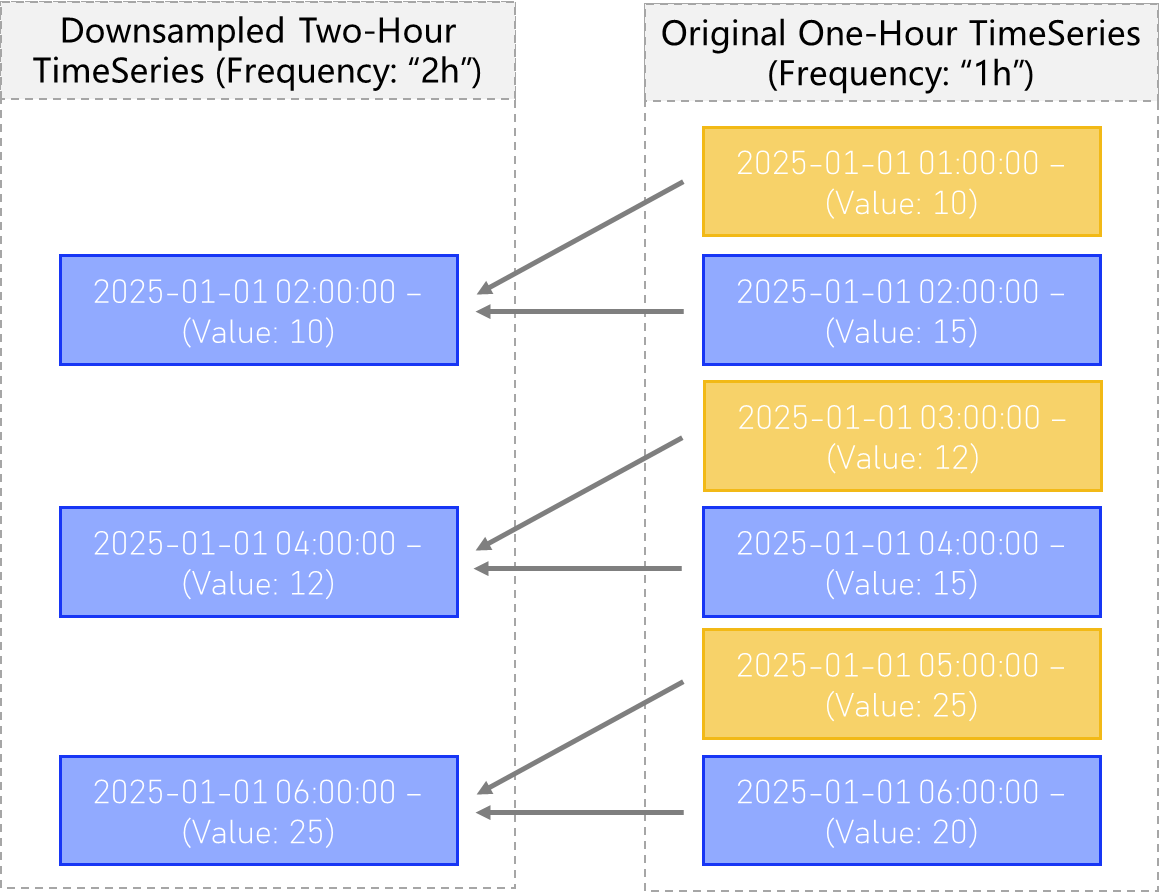
Last
The “Last” downsample setting will tell the downsampler to only use the last observed value, functioning as the opposite of the “first” setting above. This will only use the last / most recent observed value, of all the timestamp values observed in the old time bins, and assign that value to the new bin without considering any previous values.
This downsampling procedure can be visualized below:
Mechanics of Downsampling
To create a new, downsampled version of an existing TimeSeries object, you must invoke the downsample() method on an existing TS, which acts like a factory method for this specifc use case, and returns your new downsampled timeseries.
This method automatically sets many of the normally customizable attributes of TimeSeries objects, and will therefore raise an error if any of the following attributes are passed to downsample:
‘series_type’
‘underlying’
‘regular’
‘computed’
‘compute_type’
‘compute_params’
‘api_params’
‘parents’
Arguments
new_frequency: int | str – the frequency of the new TimeSeries you wish to create. This must be a valid member of the Intervals Enum class, and must correspond to a lower frequency (longer amount of time) than the parent TimeSeries.
how: str – the downsample type you wish to use. Must be a valid member of Downsample Types
**kwargs – here you can pass any additional arguments (like “name” for instance), from the “create” factory method, provided they are not listed above on the inherited attributes list.
# Import required objects
from ursa_sync.backend import TimeSeries
from ursa_sync import session

# Open a session with the database
db = session()

# Grab the first random timeseries returned with a 1-minute frequency
TS_1m = TimeSeries.load_by(['frequency'], ['1m'], db)[0]

TS_1h = TS_1m.downsample(
    new_frequency='1h',
    how='mean',
    name=f"{TS_1m} 1h downsample"
)

TS_1h.save()

# Add any tags which will help you to find this TimeSeries later on.
TS_1h.add_tags(
    "downsampled",
    "1h",
    "computed",
    "Experiment 1"
)
Rolling Metrics
Rolling Metrics like the popular Moving Average, (otherwise known as Rolling Mean), are TimeSeries metrics of critical importance in data analysis.
ursa supports the creation of rolling metric TimeSeries which are created as children of a parent TimeSeries.
Multiple rolling metrics are supported:
Rolling Mean
Rolling mean, or moving average, provides a way to compute for each timestamp, the average of the previous n timestmaps in the same series.
See the figure below:
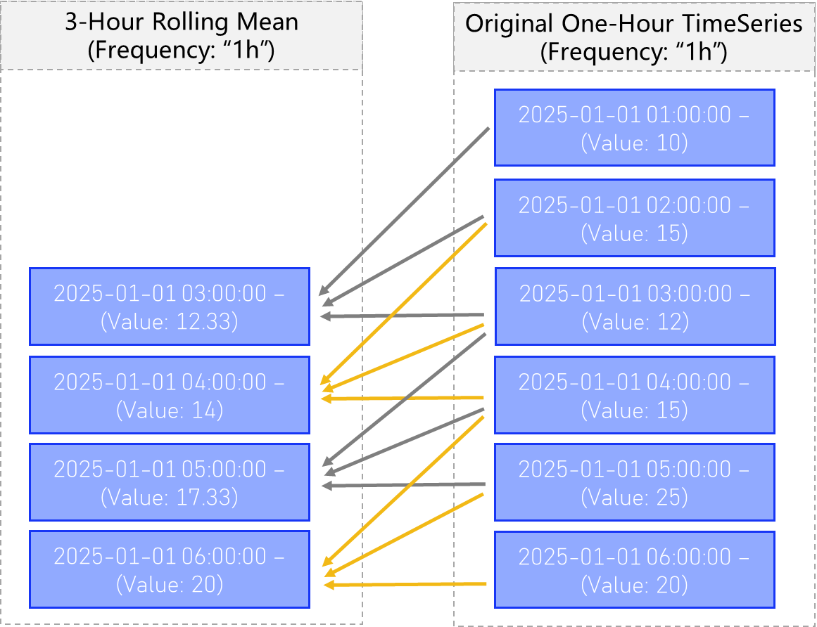
One can easily create a rolling mean child TimeSeries of a parent Series by invoking the function TimeSeries.rolling_mean()
# Import required objects
from ursa_sync.backend import TimeSeries
from ursa_sync import session

# Open a session with the database
db = session()

# Grab a random TimeSeries from the database with 1-minute frequnecy
TS = TimeSeries.load_by(['frequency'], ['1m'], db)[0]

TS_10m_rolling = TS.rolling_mean(
    window = 10
)

TS_10m_rolling.save()
The new TimeSeries dataset can be immediately queried, referenced and used:
TS_10m_rolling.dataset()
Out:
1629612000    0.374540
1629612060    0.950714
1629612120    0.731994
1629612180    0.598658
1629612240    0.156019
...
1630192040    0.857656
1630192100    0.897509
1630192160    0.946708
1630192220    0.397488
1630192280    0.217140
Length: 10000, dtype: float64
Don’t forget to close your database sessions!
db.close()
Rolling Median
Rolling Median functions identically to the Rolling Mean function, replacing the rolling computation with median instead of mean. It can be invoked with:
TS_10m_rolling = TS.rolling_median(
    window = 10
)
for more specific details about rolling metrics please see the description in the Rolling Mean section.
Rolling Standard Deviation
Rolling Standard Deviation functions identically to the Rolling Mean function, replacing the rolling computation with standard deviation instead of mean. It can be invoked with:
TS_10m_rolling = TS.rolling_std(
    window = 10
)
for more specific details about rolling metrics please see the description in the Rolling Mean section.
Exp. Rolling Mean
Exponential Rolling Mean functions identically to the Rolling Mean function, replacing the rolling computation with exponential rolling mean, instead of the normal mean. It can be invoked with:
TS_10m_rolling = TS.exp_rolling_median(
    window = 10
)
for more specific details about rolling metrics please see the description in the Rolling Mean section.
Cumulative Metrics
Cumulative metrics function like rolling metrics, but
Cumulative Sum
The Cumulative Sum is a rolling metric which computes for timestamp n, the sum of all entries for timestamp 1 to n for some parent TimeSeries. It can be invoked like this:
TS_cumsum = TS.cumsum()
TS.save()
And that’s it! The dataset is also immediately available for your new TimeSeries.
Cumulative Product
The Cumulative Product is a rolling metric which computes for timestamp n, the product of all entries for timestamp 1 to n for some parent TimeSeries. It can be invoked like this:
TS_cumprod = TS.cumprod()
TS.save()
And that’s it! The dataset is also immediately available for your new TimeSeries.
Log
The Natural Log is also an important function in all areas of Finance and Mathematics.
You can easily create new TimeSeries objects which are the natural log of a parent TimeSeries.
This can be accomplished with:
# Import required objects
from ursa_sync.backend import TimeSeries
from ursa_sync import session

# Open a session with the database
db = session()

# Grab a random percent change of closing price TimeSeries in our database:
TS_parent = TimeSeries.load_by(['series_type'], ['close_percent_change'], db)[0]

# Create a new child TimeSeries
TS_log = TS_parent.log()

# Save our new timeseries object so it persists beyond this session.
TS_log.save()

# Always close your database sessions!
db.close()
Percent Change
measures the change between some timestamp n entries ago, and now, measured as a percentage of older timestmap.
Child TimeSeries of Percent change can be created by invoking TimeSeries.pchange() as below:
# Import required objects
from ursa_sync.backend import TimeSeries
from ursa_sync import session

# Open a session with the database
db = session()

TS = TimeSeries.load_by(['frequency'], ['1m'], db)[0]

TS_pchange_10m = TS.pchange(
    window: int = 10  # The number of timestamp distances between which to compute percent change
)
X-Weights
X-Weights provide an interface for a relative comparison of any combination of TimeSeries which share a same frequency.
X-Weights creates a new TimeSeries, which is a child of one main parent, and a group of other parents whose sum we compare to our main parent.
For example, suppose we want to create a timeseries to answer the question “What percent of the crypto market cap belongs to ETH” live.
We could construct an x_weights child of Ethereum, and the other crypto asset marketcaps in the database. This creates a TimeSeries which can take on values between 0 and 1, giving the percentage market cap for Ethereum compared with the sum of all market caps of the other crypto assets.
For instance:
# Import required objects
from ursa_sync.backend import TimeSeries
from ursa_sync import session

# Open a session with the database
db = session()

ethereum = Underlying.load_by(
    ['asset_ticker'],
    ['ETH'],
    db
)

# Get all the 1d market-cap crypto parent TimeSeries objects in our database
TSS = TimeSeries.query_by_tags(
    ['market_cap', 'crypto', 'non-computed', '1d'],
    db
)

... # Here you might want to check that TSS really contains the TimeSeries objects you want.

# Now we grab the main TimeSeries to weight: Ethereum Market Cap
TS = TimeSeries.load_by(
    ['series_type', 'underlying_id', 'frequency'],
    ['market_cap', ethereum.id, '1d'],
    db
)

X_Weights = TimeSeries.x_weights(
    subject=TS,
    objects=TSS
)

X_Weights.save()
Intervals
Intervals are meant to represent the distance between two points in time, always measured in milliseconds.
Intervals are what we use any time a “frequency” is required. ursa contains a built-in Enum Class of all supported Intervals.
from ursa_sync.backend.cases.Intervals import Invervals

print(Intervals.intervals)
Out:
{
    '1ms' : 1,
    '10ms' : 10,
    '100ms' : 100,
    '1s' : 1000,
    '10s' : 10000,
    '1m' : 60000,
    '5m' : 300000,
    '10m' : 600000,
    '15m' : 900000,
    '30m' : 1800000,
    '1h' : 3600000,
    '2h' : 7200000,
    '4h' : 14400000,
    '8h' : 28800000,
    '12h' : 43200000,
    '1d' : 86400000,
    '1w' : 604800000,
    '1M' : 2592000000,
    '1Q' : 7776000000,
    '1Y' : 31536000000,
}
Here you can see the various intervals supported by ursa’s backend, and the corresponding number of milliseconds they each refer to.
The interval class also provides an interface for easily going between the two:
print(Intervals.get('1m'))
Out:
60000
print(Intervals.get_frequency(300000))
Out:
"5m"